


Introduction
In cooperation with the Robert Bosch GmbH, the Heidelberg Collaboratory for Image Processing provides some tools for the visualization of dense correspondences as they are estimated by stereo and optical flow algorithms. The visualizations have been realized in MATLAB and C++ and can be downloaded for research purposes under GNU public license. Tools for outlier-visualization on the one hand and fine-scale correspondences visualization on the other hand are implemented. Using fixed thresholds visual comparison of different algorithms also on real world scenes are possible. Additionally, we provide color-legends that allow for a one-to-one mapping between colors and estimated correspondences. The choices for designing the tools are motivated in this document [pdf].Code
We provide a package containing the C++ and MATLAB code.This package includes examples for the application of the toolbox and for the gerenration of the color-maps.
When using this code please note the disclaimer within the software.
Color Maps
The use of fixed thresholds allows for inter-algorithm comparisons and also to provide fixed color-maps for disparity and optical flow.
Figure 1: The legend for stereo visualization shows that objects with large disparity are encoded in reddish colors while objects with zero disparity are encoded in blue.
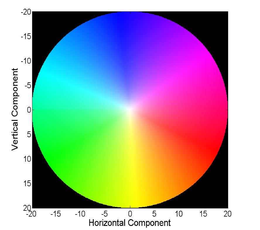
Figure 2: The legend for optical visualization shows how direction is mapped to color and magnitude is mapped to saturation.
Stereo Visualizations
For stereo we implemented three methods of visualization.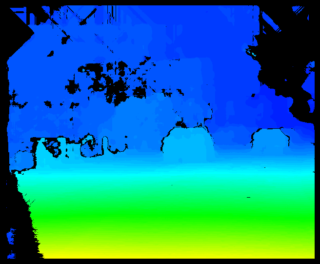
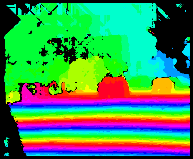
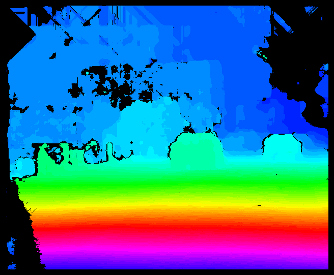
Figure 3: The fixed scaling (left) allows for comparable visualization, but does not exploit the full color-space. Cyclic encoding (middle) highlights small variations of the correspondences but gives a poor overview. Stretching between the minimal and maximal disparity, i.e. between 1 and 64 in this case, (right) allows to exploit the color-space more thoroughly but looses interpretability with the color map.
These visualizations can be combined to an overlay image that allows to visualize object boundaries and correspondence discontinuities simultaneously.
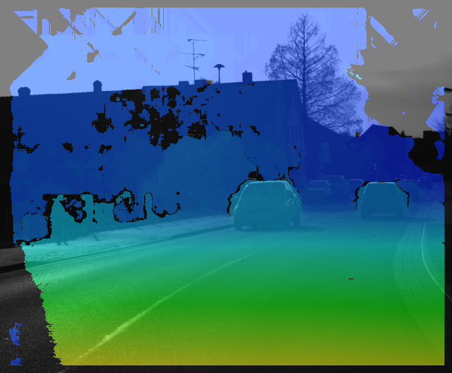
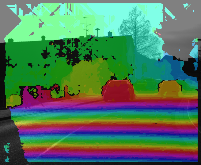
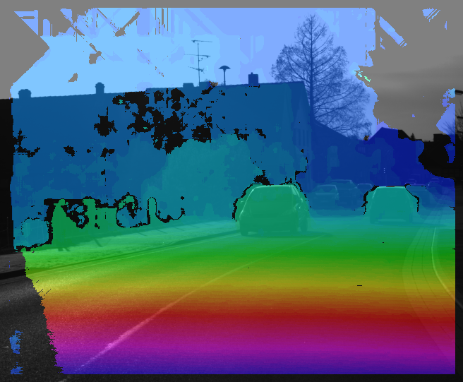
Figure 4: Overlay of correspondence visualizations and reference images.
Optical Flow Example Visualizations
For optical flow we implemented three methods of visualization.
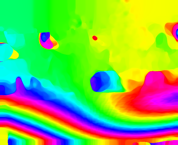
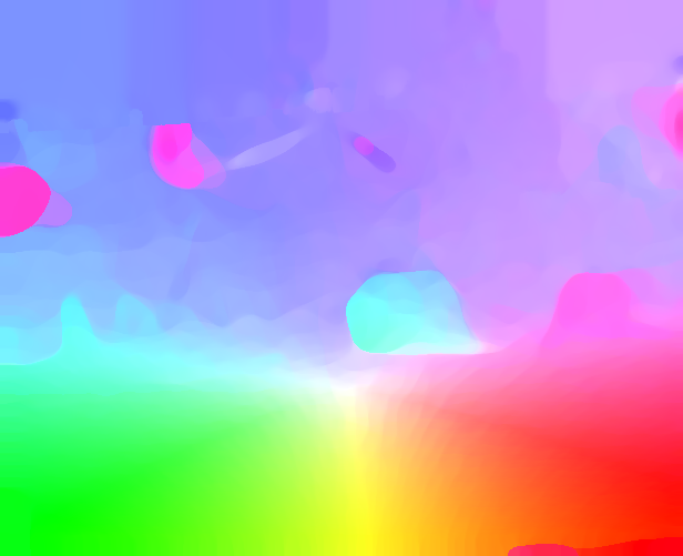
Figure 5: The fixed scaling (left) allows for comparable visualization, but does not exploit the full space of color and saturation. Cyclic encoding (middle) highlights small variations of the correspondences but gives a poor overview. Adjusting be the component mean of the flow field, i.e. by -8.60 and 2.96 in this case, (right) allows to exploit the color-space more thoroughly but looses interpretability with the color map.
These visualizations can be combined to an overlay image that allows to visualize object boundaries and correspondence discontinuities simultaneously. However, in this case variations in saturation can be due to variations in the magnitude of the flow or variations in the image.
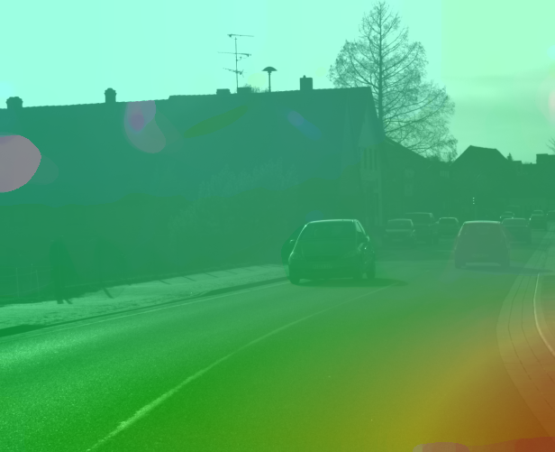
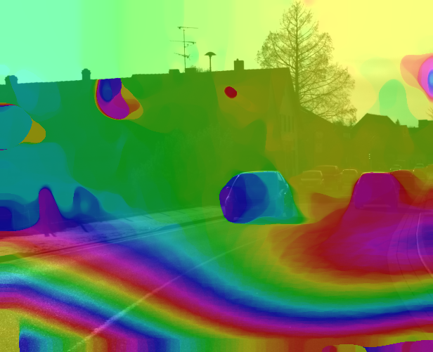
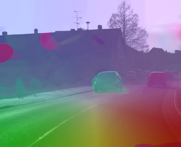
Figure 6: Overlay of correspondence visualizations and reference images.